Understanding Gradient Descent
14 min read

Machine Learning (ML) and Artificial Intelligence (AI) relies heavily on this very intuitive differentiation-based algorithm called gradient descent. It gets us closer to our desired minima or maxima by starting with a value and adjusting that value based on the change of our gradient. In this article you'll learn to understand what is gradient descent and all the component apart of it. And then explore a few modifications of it from simple to advanced to solidify your understanding!
Foreword
This article assumes understanding what a derivative is!
This remarkably simple but powerful algorithm stands on the shoulders of differentiation and is the backbone for “backward propagation of errors” (back prop) which calculates the gradients needed for gradient descent.
A quick little TLDR refresher for those who need it. The derivative at a point gives the slope of the tangent line at that point. This slope represents the rate of change of the function at that specific point. We calculate the derivative (or gradient for multivariable functions) at the current point to get the direction of the steepest ascent and make it negative to minimise the function. We iteratively recalculate the derivative/gradient at the new point and continue to adjust our input variables.
When we take a derivative and our tangent is between 0 and 180 degrees then there is a slope either slanted, either left or right, or it’s horizontal, indicating we’re at the most optimal value for the local min/max. If it’s slanted the goal is to get it closer to being horizontal/the value 0.
Single Variable
If want to minimise the value of a single variable function we would use single-variable gradient descent, denoted as
where (or ) is the step size: how much we adjust our current position to the slope/gradient we calculated from the derivative (which “nabla” aka “del” in multi-variable gradient descent, , which we’ll talk about soon). We use a negative sign to turn the ascent of the gradient into descent.
Example
Lets do a quick example to demonstrate w/ :
- The derivative is
- Starting point
- Learning step rate
- Our starting based off is
When we plug our values into our formula on iteration 0 of we get:
- Into the derivative
- Then plugging into our gradient descent
- Our new with is
- We started with and our descent step gave us so we have change in which resulted in a reduction causing a convergence to the minimum (secretly ).
The next iteration (1)
- Our starting point is updated from our previous iteration from to , PROGRESS!
- Calculate the new derivative
- Plug into gradient descent
- And calculating our output another reduction of
Then this process is repeated until we reach the minimum of the function (), aka the vertex of the parabola, with very small improvements the closer we get. So it’s really not too worth doing more iterations past a certain point because the diminishing returns become super high.
But what if we overshoot our learning rate ()?
Let’s say we fuck up our learning rate to something like as an extreme example instead of our 0.1 in iteration (1). So instead of a normal learning rate w/ we replace the 0.1 with 0.5
So our gradient went negative! This means it’s flipped from slanting one way to another. But it’s okay! It’s simply gone to the other side of the curve since it’s a parabola. Although if this was a non-convex function this may have gone into another local valley entirely! In our case it’s gone on the other curved part of the parabola and has gone down still by , so we still improved!
If the learning rate was with then we would be going back up the curve, the opposite direction to where we want to go so the learning rate needs some adjustment.
Multi-Variable
Let’s learn about the next evolution of it with the multi-variable version,
where “nabla” is added, which is commonly used in multi-variate calculus to represent a vector (one dimensional array; a matrix is multi-dimensional) of all partial derivatives, i.e., and for an example the function
the gradient would be
because we treat the terms without the variable we differentiate with respect to as constants and thus equal zero, e.g., because is the equivalent as a constant term like the number 5.
This is what we call the gradient of f — a vector of partial derivatives pointing in the direction of the steepest ascent. Gradient descent uses the negative of the gradient.
You can then adapt the gradient to whatever you like, e.g., selective learning rates for different partials based on their correlational strength to moving the needle or adding some kind of momentum factor like taking large learning steps and then slowing down as your angle gets closer to horizontal. Let’s look at a neat adaption!
Non-convex Problem
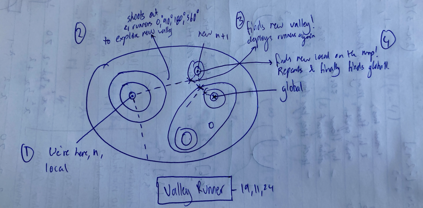
There is a big problem though non-linear problems (non-convex) because there will be many valleys and troughs, meaning there are local highs and lows and we’ll get stuck in them. Therefore, techniques to break out of these local spots are needed!
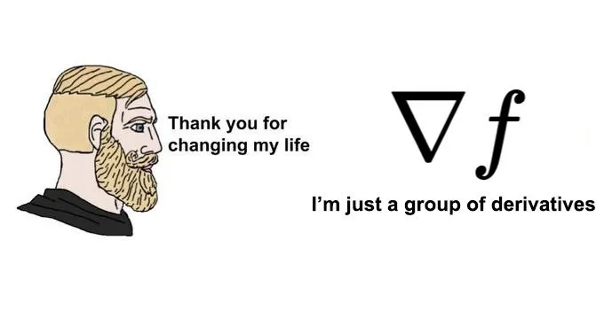
I thought of this algorithm while writing this article. Although kind of flawed it is quite interesting to explore down the road. Up next we’ll look into modifying the gradient descent algo to account for interesting enhancements, similar to what you see with this image!

Augmenting Gradient Descent Template
And so, we can extend the multi-variate gradient descent (GD), like programming, into a scaffolded version to account for automatic adaptability, meaning it has the framework for it but it’s not natively built in! It also doesn’t have an objective function to actually optimise for, which we’ll add later.
Ok, so this is a whole lot more than the previous gradient descent but I promise it’s quite intuitive! We’ll go through each colour step by step, from the inequality (green), the proposed gradient adjustment (red) and the descent redirection (blue) to make sure we understand each component of the spooky scary equation.
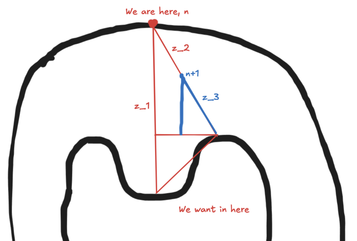
The whole idea of this modified gradient descent is to account for the assumption that the steepest descent isn’t always the best decision as it can take longer to reach the next optimal set than taking a less steep route, e.g., going sideways for a bit may end up unlocking a faster path than going straight down.
Here’s a simplified image of what I mean.

would have been our direct path to the subset but there is clearely a faster path that diverges from the tangent going vertically down so we adjust our search direction to go down ! This is an oversimplified drawing but there will be times where you need to horizontal to reach the fastest path — see how this seems counter-intuitive at first? This is what this template aims to scaffold for us.
Inequality Check
So the inequality is simply saying the next step in our descent must decrease from the current step, quite simple. You may have noticed that is replaced with . This is just a notation difference but typically is used in numerics to represent an approximation point that we update iteratively over an exact or deterministic point.
Proposed Gradient Adjustment
looks like our multi-var GD but with 3 modifications.
Dynamic Learning Rate
The first is the addition of the subscript for our learning rate which allows us to adjust our learning rate with each iteration (automatically adjusting it requires implementation though!).
Gradient Magnitude
The second is the addition of the encapsulating and — this is the Lebesgue 2 (L2) norm, denoted as which converts the multi-dimensional gradient vector into the magnitude, a single scalar value. The magnitude of the vector is useful because it measures the overall gradient sensitivity to inputs. The gradient vector itself gives the direction of the steepest descent, while its L2 norm indicates how steep that descent is. It’s like finding the slope while accounting for all the partial derivatives. It smooths out the sum, by squaring each item, enabling it to be differentiable everywhere except at the origin (bottom of the curve and therefore horizontal)!
TLDR; the gradient itself provides both direction and magnitude from the individual partial derivatives but the L2 norm gives us the overall magnitude in a single scalar value making it easier to adjust the step size computation (since we deal with one value instead of partial derivatives and the calculations associated with them).
Remember is a ‘V’ shaped graph, the square makes it like a parabola-like graph. We square our summed values because they introduce nice to work with properties like removing negative numbers and reducing the impact by smoothing the graph, relative to not squaring, making it easier to differentiate.
Descent Direction Template
The last addition is represents the descent direction at iteration which allows for the learning rate to change with each iteration to adapt the optimisation process. It can incorporate information from previous iterations or use second-order information about the function to potentially converge faster, e.g., a momentum-based method, or avoid local minima, e.g., adjacent replicas that use large learning rates to double-check if there are neighbouring valleys.
The L2 norm is also applied to because it scales the step size based on both the gradient magnitude and the magnitude of the chosen descent direction.
Momentum Example
Let’s do a quick example of a single-var momentum model to simplify the calculations and maximise the understanding. This algo is great for skipping past small local minima potholes.
We first have a simple quadratic fn and our init params are:
- Init input
- Learning rate
- Momentum
- Velocity
Before we start our first iteration consists of
- Gradient
- We then use the to update our velocity where
- is the exponential decay which ensures past velocities exponentially decay over time making recent gradients have more of an impact over older versions
- makes sure the added velocity to the gradient doesn’t grow too big, like a scale limit guardrail to make Then we update our to
So really what happening is our learning rate is influenced by our velocity which is adapts exponentially if the direction are consecutive with each iteration.
If we didn’t use the momentum factor then
Where the result would have been instead of the momentum’s . Now this is important! Since it’s an exponential function the early iterations are worse than regular gradient descent because it hasn’t accumulated any momentum from previous steps to scale it up. However, this trade-off of slow starts for potentially better long-term performance is a consideration to make.
Maybe down the line future me can write an example in Python to show the impact visually after iterations (sorry, reader-kun)
Descent Redirection
The third “scary” part of the equation is The TLDR for quick reference is that is the direction we want to descend and we modify our direction by where our gradient is. This is calculated by getting the highest possible result (using ) from all real numbers 0 to 1 where is the iteration and the input for the sensitivity of our new gradient adjustment.
Now let’s do the long-winded descriptive component analysis…
Descent Direction Vs Gradient
First we want to deal with this big fuck off part of the formula,
The numerator
is measuring the difference between the two gradients:
- At a point along the proposed step direction where is a fraction of the step, a point along the path of the proposed step. The adjustment is caused by the current gradient being moved by the descent direction scaled by the step size.
- And at the current point
The L2 norm is used once again to ensure it’s within certain bounds, which are inherited from the assumption that our formula incorporates Lipschitz continuity.
Let’s break it down.
Our numerator assumes it’s within the bounds of the maximum change of our descent direction
where is the Lipschitz constant which represents the maximum rate of change of the gradient, ensuring convergence of the gradients.
means the function’s max change is as fast as its input, it changes faster tan the input and vice versa for less than. However, is often unknown and needs to be accounted for in the step size (another thing to implement, I’m sorry).
Therefore, our rate of change is bounded by the size of the step we’re taking in our desired direction and the constant.
as it’s a property of norms.
is saying the L2 norm magnitude difference of the descent direction gradient relative to the actual gradient — so essentially trying to align the current gradient to our desired direction.
The denominator
is normalising the value by dividing the change in gradient by the magnitude of the current gradient to make the measure independent of the scale of the gradient — it essentially outputs how much of a relative change it is rather than absolute change. Think of it like when you take the mean: you sum everything up then divide by the amount of items to normalise it.
Who’s Max?
I’m going to skip the just for some context of what it’s subtracting, so bear with me. This subtraction part is quite computationally expensive because of the . It is a for loop that chooses the maximum value change of the gradient relative to it’s starting value from the formula
So it’s iterating over all real numbers from , e.g., , storing the highest possible angle change relative to the initial magnitude and then outputting the stored best one, e.g., a 35.78% change.
In practice, we don’t check every possible value in due to computational constraints with the machine but you could add precision bounds to the formula, but there is none in the one we’re looking at.
Cos Sine Sucks
Now back to the . We use this angle to measure the alignment between our two vectors: the custom descent direction (where we want the gradient to go) and the best relative negative gradient we calculated from ‘ing (we use a negative sign because we want to descend instead of ascend).
The reason why is used instead of is that cosine 1 represents perfect alignment whereas represents perpendicularity (90 degrees), which is not important for us — alignment provides more information. After all, the slightest difference tells us the slightest misalignment to adjust to realign, aka our objective to align our model. So if our is significantly less than 1 then we would inflate our step size because a small step may not provide any real results, unless there was a miraculous tiny pothole with a god value.
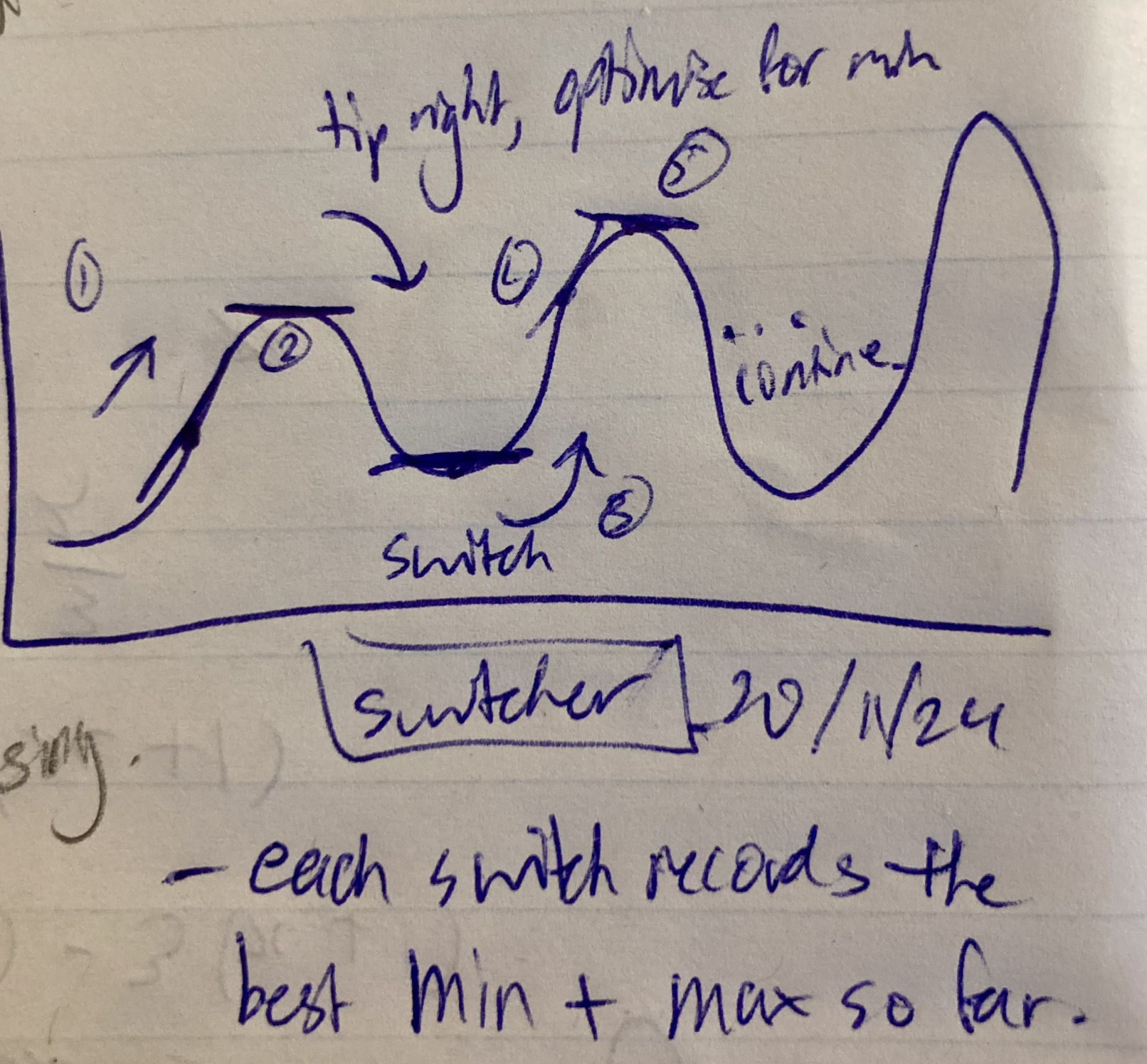
Switcher Algo Idea
While writing about the “Descent Direction” part a bit earlier in the article I thought about this simple algo that switches its objective from descent to ascent and vice versa in the opposite direction it came from once it reaches its goal. The reason for it is so it can build a mental map of the landscape if it’s a completely blackbox environment with no prior knowledge of the graph. Then it can estimate the graph using splines and/or a power series. Thought it was a cool idea to share :)

Objective Function
The objective function is the variable of the thing you’re quantitatively trying to maximise (or minimise). It can include the cost function, weights, and additional terms. If you had a square the area would be what you’re trying to optimise for or maximum profit = revenue - costs. The goal is to find the values that result in the best value of the objective function. You can even have multi-objective functions which stem into the world of Pareto optimality which refers to getting to a state where resources are allocated in the most efficient way possible so that it’s impossible to make any one party better off without making at least one other party worse off.
So basically this objective function becomes the thing the gradient descent is trying to optimise and that’s kind of the basis of ML/AI.
Loss + Cost Function
The loss function evaluates the error of a model on a single data point, typically focusing solely on the prediction error, denoted as where is the actual value and is the predicted value. It is usually calculated many times for each cycle for every data point.
The cost function is the average error for a set of data points, instead of one single point. It is calculated once each cycle. So it’s like the mean of all the loss functions.
Final
Thank you for reading my first real breakdown of, what I consider to be, foreign advanced math. I know it got a bit abstract towards the end without any real numerical examples — I just yoinked it from the wiki here. I was curious about how it worked without looking at any explanations and it turned out I learned quite a lot from just breaking it down. Hopefully, this will inspire some people or give neat ideas to others interested in this stuff.
This was actually quite challenging to break down (and I’m not even sure I did a good job tbh) but I learned a lot and hopefully you did too. I plan to make more intuition-based articles as I progress further in math, so be on the lookout for them :)
But until next time, Godspeed, anon.
Share this Article
Recent Articles
-

Overcoming Mental Warfare
When does pain stop? This constant back and forth of two titans colliding conscious never seens to let up...Will I ever escape? I must confront them, even if it means I will lose myself in the process. Fear not death but to live a life with undecisiveness.
-

Numbing Persistance
There is nothing you can do but endure and persist to grasp those dreams from many moons ago. It feels mind numbing, all this effort. Maybe one day you'll reach it but at what cost? Was it worth it? All that pain and suffering, for what cause? Are you fighting to survive or is this thought play for you? For me, it's survival. Without it I would have nothing, but to rot in my mind as time drifts by.
-

A Warrior's Journey
Deciding to become who you want to be is no easy feat. You are destined to battle the strongest of enemies on that path, sometimes with friends but majority of the time alone. What does the mind of one that is walking this path for the second time look like?
